Configuring Programs#
In this chapter, we’ll explore a number approaches for configuring our Zipf’s Law project, and ultimately decide to apply one of them.
That project should now contain:
zipf/
├── .gitignore
├── CONDUCT.md
├── CONTRIBUTING.md
├── LICENSE.md
├── Makefile
├── README.md
├── bin
│   ├── zipf.ipynb
│   ├── collate.py
│   ├── wordcount.py
│   ├── plotcount.py
│   ├── template.py
│   └── zipftest.py
├── data
│   ├── README.md
│   ├── dracula.txt
│   └── ...
└── results
    ├── collate.csv
    ├── collate.png
    ├── dracula.csv
    ├── dracula.png
    └── ...
Be Careful When Applying Settings outside Your Project
This chapter’s examples modify files outside of the Zipf’s Law project in order to illustrate some concepts. If you alter these files while following along, remember to change them back later.
Configuration File Formats#
Programmers have invented far too many formats for configuration files; rather than creating one of your own, you should adopt some widely used approach. One is to write the configuration as a Python module and load it as if it was a library. This is clever, but means that tools in other languages can’t process it.
A second option is Windows INI format, which is laid out like this:
[section1]
key1=value1
key2=value2

[section2]
key3=value3
key4=value4
INI files are simple to read and write, but the format is slowly falling out of use in favor of YAML. A simple YAML configuration file looks like this:
# Standard settings for thesis.
logfile: "/tmp/log.txt"
quiet: false
overwrite: false
fonts:
- Verdana
- Serif
Here,
the keys logfile, quiet, and overwrite
have the values /tmp/log.txt, false, and false respectively,
while the value associated with the key fonts
is a list containing Verdana and Serif.
For more discussion of YAML, see ChapterYAML.
Matplotlib Configuration#
To see overlay configuration in action, let’s consider a common task in data science: changing the size of the labels on a plot. The labels on our Jane Eyre word frequency plot are fine for viewing on screen (Figure Config Jane Eyre Default), but they will need to be bigger if we want to include the figure in a slideshow or report.
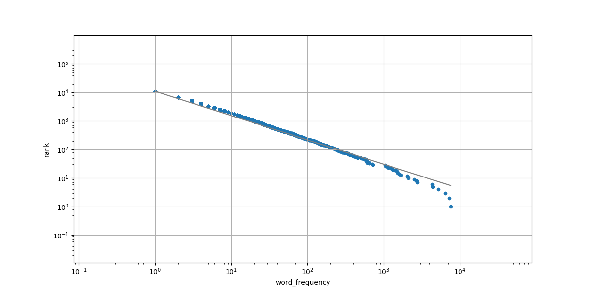
Fig. 55 Configuration example Jane Eyre#
We could use any of the overlay options described above to change the size of the labels:
Edit the system-wide Matplotlib configuration file (which would affect everyone using this computer).
Create a user-specific Matplotlib style sheet.
Create a job-specific configuration file to set plotting options in
plotcounts.py.Add some new command-line options to
plotcounts.py.
Let’s consider these options one by one.
The Global Configuration File#
Our first configuration possibility is to edit the system-wide Matplotlib runtime configuration file. When we import Matplotlib, it uses this file to set the default characteristics of the plot. We can find it on our system by running this command:
import matplotlib as mpl
mpl.matplotlib_fname()
If, for example, you use Anaconda the location could be as follows:
/Users/amira/anaconda3/lib/python3.7/site-packages/matplotlib/
mpl-data/matplotlibrc
All the different Python packages installed with Anaconda
live in a python3.7/site-packages directory,
including Matplotlib.
If not using Anaconda your output could look instead like this:
/home/nibe/.local/lib/python3.12/site-packages/matplotlib/mpl-data/matplotlibrc
matplotlibrc lists all the default settings as comments.
The default size of the X and Y axis labels is “medium”,
as is the size of the tick labels:
#axes.labelsize    : medium  ## fontsize of the x and y labels
#xtick.labelsize   : medium  ## fontsize of the tick labels
#ytick.labelsize   : medium  ## fontsize of the tick labels
We can uncomment those lines and change the sizes to “large” and “extra large”:
axes.labelsize     : x-large  ## fontsize of the x and y labels
xtick.labelsize    : large    ## fontsize of the tick labels
ytick.labelsize    : large    ## fontsize of the tick labels
and then re-generate the Jane Eyre plot with bigger labels (Figure JE Labels):
$ python bin/plotcounts.py results/jane_eyre.csv --outfile
  results/jane_eyre.png
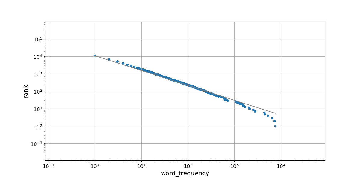
Fig. 56 Jane Eyre Config labels#
This does what we want,
but is usually the wrong approach.
Since the matplotlibrc file sets system-wide defaults,
we will now have big labels by default for all plotting we’ll do in the future,
which we may not want.
Secondly,
we want to package our Zipf’s Law code and make it available to other people (Chapter packaging).
That package won’t include our matplotlibrc file,
and we don’t have access to the one on their computer,
so this solution isn’t as reproducible as others.
A global options file is useful, though.
If we are using Matplotlib with LaTeX to generate reports
and the latter is installed in an unusual place on our computing cluster,
a one-line change in matplotlibrc can prevent a lot of failed jobs.
The User Configuration File#
If we don’t want to change the configuration for everyone, we can change it for just ourself. Matplotlib defines several carefully designed styles for plots:
import matplotlib.pyplot as plt
print(plt.style.available)
['Solarize_Light2', '_classic_test_patch', '_mpl-gallery', '_mpl-gallery-nogrid', 'bmh', 'classic', 'dark_background', 'fast', 'fivethirtyeight', 'ggplot', 'grayscale', 'seaborn-v0_8', 'seaborn-v0_8-bright', 'seaborn-v0_8-colorblind', 'seaborn-v0_8-dark', 'seaborn-v0_8-dark-palette', 'seaborn-v0_8-darkgrid', 'seaborn-v0_8-deep', 'seaborn-v0_8-muted', 'seaborn-v0_8-notebook', 'seaborn-v0_8-paper', 'seaborn-v0_8-pastel', 'seaborn-v0_8-poster', 'seaborn-v0_8-talk', 'seaborn-v0_8-ticks', 'seaborn-v0_8-white', 'seaborn-v0_8-whitegrid', 'tableau-colorblind10']
In order to make the labels bigger in all of our Zipf’s Law plots,
we could create a custom Matplotlib style sheet.
The convention is to store custom style sheets in a stylelib sub-directory
in the Matplotlib configuration directory.
That directory can be located by running the following command:
mpl.get_configdir()
'/home/nibe/.config/matplotlib'
Once we’ve created the new sub-directory:
$ mkdir /home/nibe/.config/matplotlib/stylelib
we can add a new file called big-labels.mplstyle
that has the same YAML format as the matplotlibrc file:
axes.labelsize   : x-large  ## fontsize of the x and y labels
xtick.labelsize  : large    ## fontsize of the tick labels
ytick.labelsize  : large    ## fontsize of the tick labels
To use this new style,
we would just need to add one line to plotcount.py:
plt.style.use('big-labels')
Using a custom style sheet leaves the system-wide defaults unchanged,
and it’s a good way to achieve a consistent look across our personal data visualization projects.
However, since each user has their own stylelib directory,
it doesn’t solve the problem of ensuring that other people can reproduce our plots.
Adding Command-Line Options#
A third way to change the plot’s properties
is to add some new command-line arguments to plotcount.py.
The choices parameter of add_argument lets us tell argparse
that the user is only allowed to specify a value from a predefined list:
mpl_sizes = ['xx-small', 'x-small', 'small', 'medium',
             'large', 'x-large', 'xx-large']
parser.add_argument('--labelsize', type=str, default='x-large',
                    choices=mpl_sizes,
                    help='fontsize of the x and y labels')
parser.add_argument('--xticksize', type=str, default='large',
                    choices=mpl_sizes,
                    help='fontsize of the x tick labels')
parser.add_argument('--yticksize', type=str, default='large',
                    choices=mpl_sizes,
                    help='fontsize of the y tick labels')
We can then add a few lines after the ax variable is defined in plotcount.py
to update the label sizes according to the user input:
ax.xaxis.label.set_fontsize(args.labelsize)
ax.yaxis.label.set_fontsize(args.labelsize)
ax.xaxis.set_tick_params(labelsize=args.xticksize)
ax.yaxis.set_tick_params(labelsize=args.yticksize)
Alternatively,
we can change the default runtime configuration settings before the plot is created.
These are stored in a variable called matplotlib.rcParams:
mpl.rcParams['axes.labelsize'] = args.labelsize
mpl.rcParams['xtick.labelsize'] = args.xticksize
mpl.rcParams['ytick.labelsize'] = args.yticksize
Adding extra command-line arguments is a good solution
if we only want to change a small number of plot characteristics.
It also makes our work more reproducible:
if we use a Makefile to regenerate our plots (Chapter Intro to make),
the settings will all be saved in one place.
However,
matplotlibrc has hundreds of parameters we could change,
so the number of new arguments can quickly get out of hand
if we want to tweak other aspects of the plot.
A Job Control File#
The final option for configuring our plots—the one we will actually adopt in this case—is
to pass a YAML file full of Matplotlib parameters to plotcount.py.
First,
we save the parameters we want to change in a file inside our project directory.
We can call it anything,
but plotparams.yml seems like it will be easy to remember.
We’ll store it in bin with the scripts that will use it:
# Plot characteristics
axes.labelsize   : x-large  ## fontsize of the x and y labels
xtick.labelsize  : large    ## fontsize of the tick labels
ytick.labelsize  : large    ## fontsize of the tick labels
Because this file is located in our project directory
instead of the user-specific style sheet directory,
we need to add one new option to plotcount_argparse.py to load it:
parser.add_argument('--plotparams', type=str, default=None,
                    help='matplotlib parameters (YAML file)')
We can use Python’s yaml library to read that file:
def set_plot_params(param_file):
    """Set the matplotlib parameters."""
    if param_file:
        with open(param_file, 'r') as reader:
            param_dict = yaml.load(reader,
                                   Loader=yaml.BaseLoader)
    else:
        param_dict = {}
    for param, value in param_dict.items():
        mpl.rcParams[param] = value

# ... as before..

if __name__ == "__main__":
    parser = argparse.ArgumentParser(description="Process word counts and generate plots.")
    parser.add_argument("input_file", type=str,
                        help="Input file with word counts")
    parser.add_argument("output_file", type=str,
                        help="Output file or display mode")
    parser.add_argument("--limit", type=int, default=10,
                         help="Limit the number of word counts to display")
    parser.add_argument('--plotparams', type=str, default=None,
                        help='matplotlib parameters (YAML file)')
    args = parser.parse_args()

    counts = load_word_counts(args.input_file)

    # SET PLOT PARAMS
    set_plot_params(args.plotparams)

    plot_word_counts(counts, args.limit)

    if args.output_file == "show":
        plt.show()
    elif args.output_file == "ascii":
        words, counts, _ = list(zip(*counts))
        for line in plot_ascii_bars(counts[:args.limit], words[:args.limit], truncate=False):
            print(line)
    else:
        plt.savefig(args.output_file)
Summary#
Programs are only useful if they can be controlled, and work is only reproducible if those controls are explicit and shareable. If the number of controls needed is small, adding command-line options to programs and setting those options in Makefiles is usually the best solution. As the number of options grows, so too does the value of putting options in files of their own. And if we are installing the software on large systems that are used by many people, such as a research cluster, system-wide configuration files let us hide the details from people who just want to get their science done.
More generally, the problem of configuring a program illustrates the difference between “works for me on my machine” and “works for everyone, everywhere.” From reproducible workflows (Chapter make or Chapter workflows with snakemake to logging (Section Reporting Errors), this difference influences every aspect of a research software engineer’s work. We don’t always have to design for large-scale re-use, but knowing what it entails allows us to make a conscious, thoughtful choice.
Keypoints#
Overlay configuration specifies settings for a program in layers, each of which overrides previous layers.
Use a system-wide configuration file for general settings.
Use a user-specific configuration file for personal preferences.
Use a job-specific configuration file with settings for a particular run.
Use command-line options to change things that commonly change.
Use YAML or some other standard syntax to write configuration files.
Save configuration information to make your research reproducible.