Testing Software#
This chapter demonstrates software testing using two projects: the Zipf’s Law project, and the German AQI Analyzer, our second running example. Both are introduced in Chapter Getting Started.
The first sections use Zipf to introduce core concepts; the final section shows how the same concepts apply to the AQI project. Note that some tests might be applicable to one project and not the other, depending on the nature of the project itself.
Here’s the current structure of our Zipf’s Law project files:
zipf/
├── .gitignore
├── CONDUCT.md
├── CONTRIBUTING.md
├── LICENSE.md
├── README.md
├── bin
│   ├── collate.py
│   ├── wordcount.py
│   ├── plotcount.py
│   ├── plotparams.yml
│   ├── template.py
│   └── ...
├── data
│   ├── README.md
│   ├── dracula.txt
│   └── ...
└── results
    ├── collated.txt
    ├── collated.png
    ├── dracula.txt
    ├── dracula.png
    └── ...
Assertions#
The first step in building confidence in our programs is to assume that mistakes will happen and guard against them. This is called defensive programming, and the most common way to do it is to add assertions to our code so that it checks itself as it runs. An assertion is a statement that something must be true at a certain point in a program. When Python sees an assertion, it checks the assertion’s condition. If it’s true, Python does nothing; if it’s false, Python halts the program immediately and prints a user-defined error message. For example, this code halts as soon as the loop encounters an impossible word frequency:
frequencies = [13, 10, 2, -4, 5, 6, 25]
total = 0.0
for freq in frequencies[:5]:
    assert freq >= 0.0, 'Word frequencies must be non-negative'
    total += freq
print('total frequency of first 5 words:', total)
---------------------------------------------------------------
AssertionError                Traceback (most recent call last)
<ipython-input-19-33d87ea29ae4> in <module>()
      2 total = 0.0
      3 for freq in frequencies[:5]:
----> 4     assert freq >= 0.0, 'Word frequencies must be
            non-negative'
      5     total += freq
      6 print('total frequency of first 5 words:', total)

AssertionError: Word frequencies must be non-negative
Programs intended for widespread use are full of assertions: 10%–20% of the code they contain are there to check that the other 80%–90% are working correctly. Broadly speaking, assertions fall into three categories:
A precondition is something that must be true at the start of a function in order for it to work correctly. For example, a function might check that the list it has been given has at least two elements and that all of its elements are integers.
A postcondition is something that the function guarantees is true when it finishes. For example, a function could check that the value being returned is an integer that is greater than zero, but less than the length of the input list.
An invariant (in is something that is true for every iteration in a loop. The invariant might be a property of the data (as in the example above), or it might be something like, “the value of
highestis less than or equal to the current loop index.”
The function get_power_law_params in our plotcounts.py script
is a good example of the need for a precondition.
Its docstring does not say that its word_counts parameter must be a list of numeric word counts;
even if we add that,
a user might easily pass in a list of the words themselves instead.
Adding an assertion makes the requirement clearer,
and also guarantees that the function will fail as soon as it is called
rather than returning an error from scipy.optimize.minimize_scalar
that would be more difficult to interpret/debug.
def get_power_law_params(word_counts):
    """
    Get the power law parameters.

    References
    ----------
    Moreno-Sanchez et al (2016) define alpha (Eq. 1),
      beta (Eq. 2) and the maximum likelihood estimation (mle)
      of beta (Eq. 6).

    Moreno-Sanchez I, Font-Clos F, Corral A (2016)
      Large-Scale Analysis of Zipf's Law in English Texts.
      PLoS ONE 11(1): e0147073.
      https://doi.org/10.1371/journal.pone.0147073
    """
    assert type(word_counts) == np.ndarray, \
        'Input must be a numerical (numpy) array of word counts'
    mle = minimize_scalar(nlog_likelihood,
                          bracket=(1 + 1e-10, 4),
                          args=word_counts,
                          method='brent')
    beta = mle.x
    alpha = 1 / (beta - 1)
    return alpha
Update plotcount.py with the assertion described above.
You’ll see additional examples of assertions throughout this chapter.
Unit Testing#
Catching errors is good, but preventing them is better,
so responsible programmers test their code.
As the name suggests,
a unit test checks the correctness of a single unit of software.
Exactly what constitutes a “unit” is subjective,
but it typically means the behavior of a single function in one situation.
In our Zipf’s Law software,
the count_words function in wordcount.py is
a good candidate for unit testing:
def word_count(input_file, output_file, min_length=1):
    """
    Load a file, calculate the frequencies of each word in the file and
    save in a new file the words, counts and percentages of the total  in
    descending order. Only words whose length is >= min_length are
    included.
    """
    lines = load_text(input_file)
    counts = calculate_word_counts(lines)
    sorted_counts = word_count_dict_to_tuples(counts)
    sorted_counts = filter_word_counts(sorted_counts, min_length)
    percentage_counts = calculate_percentages(sorted_counts)
    save_word_counts(output_file, percentage_counts)
A single unit test will typically have:
a fixture, which is the thing being tested (e.g., an array of numbers);
an actual result, which is what the code produces when given the fixture; and
an expected result that the actual result is compared to.
The fixture is typically a subset or smaller version of the data
the function will typically process.
For instance,
in order to write a unit test for the count_words function,
we could use a piece of text small enough for us to count word frequencies by hand.
Let’s add the poem Risk by Anaïs Nin to our data:
$ cd ~/zipf
$ mkdir test_data
$ cat test_data/risk.txt
And then the day came,
when the risk
to remain tight
in a bud
was more painful
than the risk
it took
to blossom.
We can then count the words by hand to construct the expected result:
from collections import Counter


risk_poem_counts = {'the': 3, 'risk': 2, 'to': 2, 'and': 1,
  'then': 1, 'day': 1, 'came': 1, 'when': 1, 'remain': 1,
  'tight': 1, 'in': 1, 'a': 1, 'bud': 1, 'was': 1,
  'more': 1, 'painful': 1, 'than': 1, 'it': 1, 'took': 1,
  'blossom': 1}
expected_result = Counter(risk_poem_counts)
We then generate the actual result by calling count_words,
and use an assertion to check if it is what we expected:
import sys
sys.path.append('/LOCATION/.../zipf/bin')
import wordcount

lines = wordcount.load_text(test_data/risk.txt)
actual_result = wordcount.calculate_word_counts(lines)
assert actual_result == expected_result
There’s no output, which means the assertion (and test) passed. (Remember, assertions only do something if the condition is false.)
Appending the Import Path
The last code chunk included
sys.path.append, which allowed us to import scripts from elsewhere than our current working directory. This isn’t a perfect solution, but works well enough for quick tests while developing code, especially since the tool we’ll use for the rest of the chapter handles this issue for us. [Import statements][python-import] are notoriously tricky, but we’ll learn better methods for organizing our code for function imports in Chapter on Packaging.
Testing Frameworks#
Writing one unit test is easy enough, but we should check other cases as well.
To manage them, we can use a test framework
(also called a test runner).
The most widely used test framework for Python is called pytest, which structures tests as follows:
Tests are put in files whose names begin with
test_.Each test is a function whose name also begins with
test_.These functions use
assertto check results.
Following these rules,
we can create a test_wordcount.py script in your newly created test directory
that contains the test we just developed:
from collections import Counter

import wordcount


def test_word_count():
    """Test the counting of words.

    The example poem is Risk, by Anaïs Nin.
    """
    risk_poem_counts = {'the': 3, 'risk': 2, 'to': 2, 'and': 1,
      'then': 1, 'day': 1, 'came': 1, 'when': 1, 'remain': 1,
      'tight': 1, 'in': 1, 'a': 1, 'bud': 1, 'was': 1,
      'more': 1, 'painful': 1, 'than': 1, 'it': 1, 'took': 1,
      'blossom': 1}
    expected_result = Counter(risk_poem_counts)
    lines = wordcount.load_text(test_data/risk.txt)
    actual_result = wordcount.calculate_word_counts(lines)
    assert actual_result == expected_result
The pytest library comes with a command-line tool that is also called pytest.
When we run it with no options,
it searches for all files in or below the working directory
whose names match the pattern test_*.py.
It then runs the tests in these files and summarizes their results.
(If we only want to run the tests in a particular file,
we can use the command pytest path/to/test_file.py.)
$ pytest
==================== test session starts ======================
platform linux -- Python 3.12.3, pytest-7.4.3, pluggy-1.5.0
rootdir: /home/nibe/PROJECTS/zipf/
collected 1 item

test/test_word_count.py  .                                     [100%]

===================== 1 passed in 0.02s =======================
HINT: it is good practice to run pytest from the root directory, especially when tests have to access files. Running the test from the root directory allows a more straightforward path management.
To add more tests,
we simply write more test_ functions in test_wordcount.py.
For instance,
besides counting words,
the other critical part of our code is the calculation of the \(\alpha\) parameter.
Earlier we defined a power law relating \(\alpha\)
to the word frequency \(f\),
the word rank \(r\), and a constant of proportionality \(c\) :
\( r = cf^{\frac{-1}{\alpha}} \)
We also noted that Zipf’s Law holds exactly when \(\alpha\) is equal to one. Setting \(\alpha\) to one and re-arranging the power law gives us:
\( c = f/r \)
We can use this formula to generate synthetic word count data (i.e., our test fixture) with a constant of proportionality set to a hypothetical maximum word frequency of 600 (and thus \(r\) ranges from 1 to 600):
import numpy as np


max_freq = 600
counts = np.floor(max_freq / np.arange(1, max_freq + 1))
print(counts)
[600. 300. 200. 150. 120. 100.  85.  75.  66.  60.  54.  50.
  46.  42.  40.  37.  35.  33.  31.  30.  28.  27.  26.  25.
 ...
   1.   1.   1.   1.   1.   1.   1.   1.   1.   1.   1.   1.]
(We use np.floor to round down to the nearest whole number,
because we can’t have fractional word counts.)
Passing this test fixture to get_power_law_params in plotcount.py
should give us a value of 1.0.
To test this, we can add a second test to test_countwords.py:
from collections import Counter

import numpy as np

import plotcount
import wordcount


def test_alpha():
    """Test the calculation of the alpha parameter.

    The test word counts satisfy the relationship,
      r = cf**(-1/alpha), where
      r is the rank,
      f the word count, and
      c is a constant of proportionality.

    To generate test word counts for an expected alpha of
      1.0, a maximum word frequency of 600 is used
      (i.e. c = 600 and r ranges from 1 to 600)
    """
    max_freq = 600
    counts = np.floor(max_freq / np.arange(1, max_freq + 1))
    actual_alpha = plotcount.get_power_law_params(counts)
    expected_alpha = 1.0
    assert actual_alpha == expected_alpha


def test_word_count():
    #...as before...
Let’s re-run both of our tests:
$ pytest
zipf on main [✘!?] took 19s
✦ ❯ pytest
================================================================================================ test session starts ================================================================================================
platform linux -- Python 3.12.3, pytest-7.4.3, pluggy-1.5.0
rootdir: /home/nibe/PROJECTS/zipf
collected 2 items
test/test_word_count.py F. [100%]
===================================================================================================== FAILURES ======================================================================================================
____________________________________________________________________________________________________ test_alpha _____________________________________________________________________________________________________
def test_alpha():
"""Test the calculation of the alpha parameter.
The test word counts satisfy the relationship,
r = cf**(-1/alpha), where
r is the rank,
f the word count, and
c is a constant of proportionality.
To generate test word counts for an expected alpha of
1.0, a maximum word frequency of 600 is used
(i.e. c = 600 and r ranges from 1 to 600)
"""
max_freq = 600
counts = np.floor(max_freq / np.arange(1, max_freq + 1))
actual_alpha = plotcount.get_power_law_params(counts)
expected_alpha = 1.0
> assert actual_alpha == expected_alpha
E assert 0.9951524579316625 == 1.0
test/test_countwords.py:27: AssertionError
============================================================================================== short test summary info ==============================================================================================
FAILED test/test_countwords.py::test_alpha - assert 0.9951524579316625 == 1.0
============================================================================================ 1 failed, 1 passed in 0.62s ===========================================================================================
The output tells us that one test failed but the other test passed.
This is a very useful feature of test runners like pytest:
they continue on and complete all the tests
rather than stopping at the first assertion failure as a regular Python script would.
Testing Floating-Point Values#
The output above shows that while test_alpha failed,
the actual_alpha value of 0.9951524579316625 was very close to the expected value of 1.0.
After a bit of thought,
we decide that this isn’t actually a failure:
the value produced by get_power_law_params is an estimate,
and being off by half a percent is good enough.
This example shows that testing scientific software almost always requires us to make the same kind of judgment calls that scientists have to make when doing any other sort of experimental work. If we are measuring the mass of a proton, we might expect ten decimal places of accuracy. If we are measuring the weight of a baby penguin, on the other hand, we’ll probably be satisfied if we’re within five grams. What matters most is that we are explicit about the bounds we used so that other people can tell what we actually did.
Degrees of Difficulty
There’s an old joke that physicists worry about decimal places, astronomers worry about powers of ten, and economists are happy if they’ve got the sign right.
So how should we write tests when we don’t know precisely what the right answer is? The best approach is to write tests that check if the actual value is within some tolerance of the expected value. The tolerance can be expressed as the absolute error, which is the absolute value of the difference between two, or the relative error, which the ratio of the absolute error to the value we’re approximating [Goldberg, 1991]. For example, if we add 9+1 and get 11, the absolute error is 1 (i.e., \(11-10\), and the relative error is 10%. If we add \(99+1\) and get 101, on the other hand, the absolute error is still 1, but the relative error is only 1%.
For test_alpha,
we might decide that an absolute error of 0.01 in the estimation of \(\alpha\) is acceptable.
If we are using pytest,
we can check that values lie within this tolerance using pytest.approx:
from collections import Counter

import pytest
import numpy as np

import plotcounts
import countwords


def test_alpha():
    """Test the calculation of the alpha parameter.

    The test word counts satisfy the relationship,
      r = cf**(-1/alpha), where
      r is the rank,
      f the word count, and
      c is a constant of proportionality.

    To generate test word counts for an expected alpha of
      1.0, a maximum word frequency of 600 is used
      (i.e. c = 600 and r ranges from 1 to 600)
    """
    max_freq = 600
    counts = np.floor(max_freq / np.arange(1, max_freq + 1))
    actual_alpha = plotcounts.get_power_law_params(counts)
    expected_alpha = pytest.approx(1.0, abs=0.01)
    assert actual_alpha == expected_alpha


def test_word_count():
    #...as before...
When we re-run pytest,
both tests now pass:
$ pytest
==================== test session starts ======================
platform linux -- Python 3.12.3, pytest-7.4.3, pluggy-1.5.0
rootdir: /home/nibe/PROJECTS/zipf
collected 2 items

btest/test_word_count.py  ..                                    [100%]

===================== 2 passed in 0.69s =======================
Testing Visualizations
Testing visualizations is hard: any change to the dimension of the plot, however small, can change many pixels in a raster image, and cosmetic changes such as moving the legend up a couple of pixels will cause all of our tests to fail.
The simplest solution is therefore to test the data used to produce the image rather than the image itself. Unless we suspect that the plotting library contains bugs, the correct data should always produce the correct plot.
Integration Testing#
Our Zipf’s Law analysis has two steps: counting the words in a text and estimating the \(\alpha\) parameter from the word count. Our unit tests give us some confidence that these components work in isolation, but do they work correctly together? Checking that is called integration testing.
Integration tests are structured the same way as unit tests: a fixture is used to produce an actual result that is compared against the expected result. However, creating the fixture and running the code can be considerably more complicated. For example, in the case of our Zipf’s Law software, an appropriate integration test fixture might be a text file with a word frequency distribution that has a known \(\alpha\) value. In order to create this text fixture, we need a way to generate random words.
Fortunately, a Python library called
RandomWordGenerator
exists to do just that.
We can install it using [pip][pip], the Python Package Installer:
$ pip install Random-Word-Generator
Borrowing from the word count distribution we created for test_alpha,
we can use the following code to create a text file full of random words
with a frequency distribution that corresponds to an \(alpha\) of approximately 1.0:
import numpy as np
from RandomWordGenerator import RandomWord


max_freq = 600
word_counts = np.floor(max_freq / np.arange(1, max_freq + 1))
rw = RandomWord()
random_words = rw.getList(num_of_words=max_freq)
writer = open('test_data/random_words.txt', 'w')
for index in range(max_freq):
    count = int(calculate_word_counts[index])
    word_sequence = f'{random_words[index]} ' * count
    writer.write(word_sequence + '\n')
writer.close()
We can confirm this code worked by checking the resulting file:
tail -n 5 test_data/random_words.txt
lZnkzoBHRb
djiroplqrJ
HmAUGOncHg
DGLpfTIitu
KALSfPkrga
We can then add this integration test to test_wordcount.py:
def test_integration():
    """Test the full word count to alpha parameter workflow."""
    with open('test_data/random_words.txt', 'r') as reader:
        word_counts_dict = countwords.calculate_word_counts(reader)
    counts_array = np.array(list(word_counts_dict.values()))
    actual_alpha = plotcount.get_power_law_params(counts_array)
    expected_alpha = pytest.approx(1.0, abs=0.01)
    assert actual_alpha == expected_alpha
Finally,
we re-run pytest to check that the integration test passes:
$ pytest
===================== test session starts =====================
platform linux -- Python 3.12.3, pytest-7.4.3, pluggy-1.5.0
rootdir: /home/nibe/PROJECTS/zipf
collected 3 items

test/test_word_count.py ...                               [100%]

======================= 3 passed in 0.48s =====================
Regression Testing#
So far we have tested two simplified texts: a short poem and a collection of random words with a known frequency distribution. The next step is to test with real data, i.e., an actual book. The problem is, we don’t know the expected result: it’s not practical to count the words in Dracula by hand, and even if we tried, the odds are good that we’d make a mistake.
For this kind of situation we can use regression testing. Rather than assuming that the test’s author knows what the expected result should be, regression tests compare today’s answer with a previous one. This doesn’t guarantee that the answer is right—if the original answer is wrong, we could carry that mistake forward indefinitely—but it does draw attention to any changes (or “regressions”).
In Section Git advanced zipf-verify)
we calculated an \(\alpha\) of 1.0866646252515038 for Dracula.
Let’s use that value to add a regression test to test_zipfs.py:
def test_regression():
    """Regression test for Dracula."""
    with open('data/dracula.txt', 'r') as reader:
        word_counts_dict = countwords.calculate_word_countss(reader)
    counts_array = np.array(list(word_counts_dict.values()))
    actual_alpha = plotcounts.get_power_law_params(counts_array)
    expected_alpha = pytest.approx(1.087, abs=0.001)
    assert actual_alpha == expected_alpha
$ pytest
===================== test session starts =====================
platform linux -- Python 3.12.3, pytest-7.4.3, pluggy-1.5.0
rootdir: /home/nibe/PROJECTS/zipf
collected 4 items

bin/test_zipfs.py ....                                  [100%]

====================== 4 passed in 0.56s ======================
Test Coverage#
How much of our code do the tests we have written check?
More importantly,
what parts of our code \emph{aren’t} being tested (yet)?
To find out,
we can use a tool to check their code coverage.
Most Python programmers use the coverage library,
which we can once again install using pip:
$ pip install coverage
Once we have it,
we can use it to run pytest on our behalf:
$ coverage run -m pytest
===================== test session starts =====================
platform linux -- Python 3.12.3, pytest-7.4.3, pluggy-1.5.0
rootdir: /home/nibe/PROJECTS/zipf
collected 4 items

bin/test_countwords.py ....                                  [100%]

====================== 4 passed in 0.72s ======================
The coverage command doesn’t display any information of its own,
since mixing that in with our program’s output would be confusing.
Instead,
it puts coverage data in a file called .coverage (with a leading .) in the current directory.
To display that data,
we run:
$ coverage report -m
bin/wordcount.py      20      7    65%   25-26, 30-38
bin/plotcount.py      58     37    36%   48-55, 75-77, 82-83,
                                          88-118, 122-140
bin/testzipf.py      31      0   100%
-------------------------------------------------
TOTAL                 117     49    58%
This summary shows us that
some lines of wordcount.py or plotcount.py
were not executed when we ran the tests:
in fact,
only 65% and 36% of the lines were run respectively.
This makes sense,
since much of the code in those scripts
is devoted to handling command-line arguments or file I/O
rather than the word counting and parameter estimation functionality
that our unit, integration, and regression tests focus on.
To make sure that’s the case,
we can get a more complete report by running coverage html at the command line
and opening htmlcov/index.html.
Clicking on the name of our wordcount.py script, for instance,
produces the colorized line-by-line display shown in Figure python coverage.
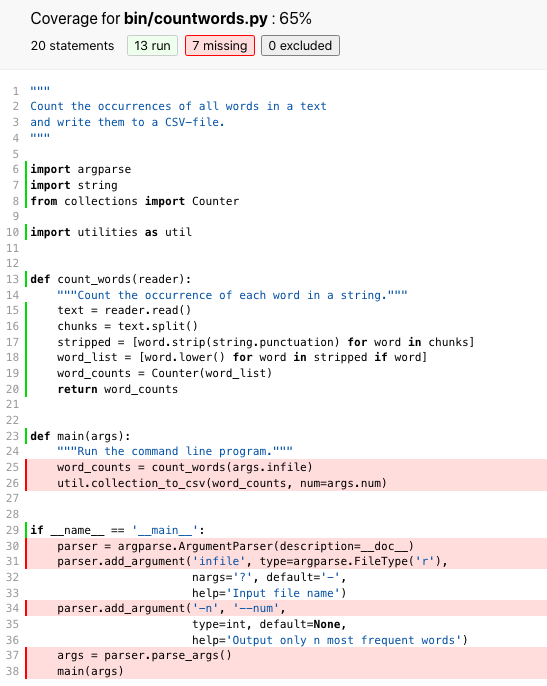
Fig. 39 Python Coverage#
This output confirms that all lines relating to word counting were tested, but not any of the lines related to argument handling or I/O.
Commit our Coverage?
At this point, you’re probably wondering if you should use version control to track the files reporting your code’s coverage. While it won’t necessarily harm your code, the reports will become inaccurate unless you continue updating your coverage reports as your code changes. Therefore, we recommend adding
.coverageandhtmlcov/to your.gitignorefile. In the next section, we’ll explore an approach that can help you automate tasks like assessing coverage.
Is this good enough? The answer depends on what the software is being used for and by whom. If it is for a safety-critical application such as a medical device, we should aim for 100% code coverage, i.e., every single line in the application should be tested. In fact, we should probably go further and aim for 100% path coverage to ensure that every possible path through the code has been checked. Similarly, if the software has become popular and is being used by thousands of researchers all over the world, we should probably check that it’s not going to embarrass us.
But most of us don’t write software that people’s lives depend on, or that is in a “top 100” list, so requiring 100% code coverage is like asking for ten decimal places of accuracy when checking the voltage of a household electrical outlet. We always need to balance the effort required to create tests against the likelihood that those tests will uncover useful information. We also have to accept that no amount of testing can prove a piece of software is completely correct. A function with only two numeric arguments has 2^128^ possible inputs. Even if we could write the tests, how could we be sure we were checking the result of each one correctly?
\newpage
Luckily, we can usually put test cases into groups. For example, when testing a function that summarizes a table full of data, it’s probably enough to check that it handles tables with:
no rows
only one row
many identical rows
rows having keys that are supposed to be unique, but aren’t
rows that contain nothing but missing values
Some projects develop checklists like this one to remind programmers what they ought to test. These checklists can be a bit daunting for newcomers, but they are a great way to pass on hard-earned experience.
Testing the AQI Project#
The same testing principles introduced above apply to the the AQI project, our second running example. The following sections walk through how each concept appears in practice.
Project Structure#
Source code lives in src/ and tests in tests/:
german-air-quality-index-analyzer/
├── src
│   ├── aqi_calculator.py
│   └── aqi_thresholds.py
├── tests
│   └── test_aqi_calculator.py
└── ...
Defensive Programming in classify_pollutant#
The core function classify_pollutant maps a single pollutant concentration
to one of five AQI categories.
It uses defensive checks to catch bad input early:
def classify_pollutant(value, pollutant):
    if value is None or pd.isna(value):
        return None                          # missing sensor reading

    if pollutant not in THRESHOLDS_BY_POLLUTANT:
        raise ValueError(f"Unknown pollutant: {pollutant}")

    for t in thresholds:
        ...

    raise ValueError(
        f"No threshold found for pollutant '{pollutant}' with value {value}"
    )
The first guard handles missing sensor data gracefully instead of crashing.
The second raises an error immediately if an unrecognised pollutant name is passed in,
rather than returning a silently wrong result.
The final raise is a postcondition:
if execution reaches that point, something is wrong with the threshold definitions themselves.
Unit Tests#
A basic unit test for classify_pollutant follows the same fixture–actual–expected pattern:
from aqi_calculator import classify_pollutant

def test_classify_pm10_good():
    assert classify_pollutant(18, "pm10") == "good"
Parametrized Tests#
Because classify_pollutant must work for five pollutants across five categories each,
pytest.mark.parametrize runs one test function across a list of cases
instead of repeating the same structure for every combination:
import pytest
from aqi_calculator import classify_pollutant

CASES = [
    ("pm10", 18,  "good"),
    ("pm10", 40,  "moderate"),
    ("pm25", 10,  "good"),
    ("o3",  100,  "moderate"),
    ("no2",  80,  "poor"),
]

@pytest.mark.parametrize("pollutant,value,expected", CASES)
def test_classify_pollutant(pollutant, value, expected):
    assert classify_pollutant(value, pollutant) == expected
Running pytest from the project root collects and runs all 58 tests across the full test file:
$ pytest tests/
============================= test session starts ==============================
platform darwin -- Python 3.12.2, pytest-7.4.4, pluggy-1.6.0
rootdir: ~/german-air-quality-index-analyzer
configfile: pyproject.toml
plugins: cov-5.0.0, hypothesis-6.131.15, anyio-4.2.0
collected 58 items

tests/test_aqi_calculator.py ...........................................  [100%]

============================== 58 passed in 0.52s ==============================
Testing for Expected Exceptions#
The defensive checks in classify_pollutant should also be tested.
pytest.raises asserts that a specific exception is raised for bad input:
def test_invalid_pollutant_raises():
    with pytest.raises(ValueError, match="Unknown pollutant"):
        classify_pollutant(10, "invalid_pollutant")
This confirms that the function fails loudly on bad input rather than silently returning a wrong category.
Equivalence Classes and Boundary Value Testing#
The AQI project uses both techniques together. Equivalence class tests check that a representative mid-range value in each category is classified correctly — the assumption being that if one value in a range works, all values in that range work:
CLASSIFY_EQUIVALENCE_CLASSES = [
    ("pm10", 5,  "very good"),   # mid-range value
    ("pm10", 18, "good"),        # mid-range value
    ("pm10", 40, "moderate"),    # mid-range value
    ...
]
Boundary value tests go further by checking the exact thresholds where one category ends and the next begins — precisely the values most likely to expose an off-by-one error:
def test_pm10_boundaries():
    assert classify_pollutant(9,  "pm10") == "very good"  # upper boundary
    assert classify_pollutant(10, "pm10") == "good"        # first value of next category
    assert classify_pollutant(27, "pm10") == "good"        # upper boundary
    assert classify_pollutant(28, "pm10") == "moderate"    # first value of next category
There is intentional overlap between the two: some values appear in both sets of tests. This is not redundancy — it is complementary coverage. Equivalence class tests verify that the classification logic works for typical inputs; boundary tests verify that the threshold definitions themselves are correct at the edges. A bug could pass one and be caught by the other.
The Rest of the Test Suite#
The full test file covers two more functions and uses class-based test organization,
grouping related tests under class TestComputeRowAqi, class TestComputeAqiForDataframe,
and class TestThresholds.
compute_row_aqi applies the max rule across all pollutants measured in one hour:
whichever pollutant falls in the worst category determines the overall AQI for that row.
Its tests verify single-pollutant cases, multiple pollutants in the same category,
multiple pollutants in different categories, and missing values —
None and NaN readings (common when a sensor is offline) must be skipped gracefully
rather than raising an error.
TestComputeAqiForDataframe serves as an integration test:
it feeds a full DataFrame through the entire pipeline —
classify_pollutant → compute_row_aqi → compute_aqi_for_dataframe —
and checks that the final output is correct end to end.
It also includes an empty DataFrame to confirm the pipeline handles that edge case
without crashing.
TestThresholds checks that the AQI_LEVELS list and AQI_SCORE dictionary
contain exactly the expected values — a simple but important safeguard,
since the rest of the logic depends on these constants being correct.
Coverage#
Running the full test suite with coverage confirms that all testable lines are exercised.
The main() function is a demonstration script that prints example output —
it is not part of the calculation logic and is not called during testing.
It is excluded from coverage with # pragma: no cover,
which is why the report reaches 100%.
$ coverage run -m pytest tests/
$ coverage report -m
Name                           Stmts   Miss  Cover
--------------------------------------------------
src/aqi_calculator.py             43      0   100%
src/aqi_thresholds.py             13      0   100%
tests/test_aqi_calculator.py     141      0   100%
--------------------------------------------------
TOTAL                            197      0   100%
Running Tests Automatically#
Running tests manually works well during development,
but it is easy to forget to run them before pushing changes.
The AQI project automates this using a CI/CD pipeline defined in a Jenkinsfile at the project root —
every time a commit is pushed, the pipeline runs the full test suite and publishes the coverage report automatically.
We will cover this in detail in Chapter CI/CD.
When to Write Tests#
We have now met the three major types of test: unit, integration, and regression. At what point in the code development process should we write these? The answer depends on who you ask.
Many programmers are passionate advocates of a practice called test-driven development (TDD). Rather than writing code and then writing tests, they write the tests first and then write just enough code to make those tests pass. Once the code is working, they clean it up (Chapter readable code) and then move on to the next task. TDD’s advocates claim that this leads to better code because:
Writing tests clarifies what the code is actually supposed to do.
It eliminates confirmation bias. If someone has just written a function, they are predisposed to want it to be right, so they will bias their tests towards proving that it is correct instead of trying to uncover errors.
Writing tests first ensures that they actually get written.
These arguments are plausible. However, studies such as [Fucci et al., 2016] and [Fucci et al., 2017] don’t support them: in practice, writing tests first or last doesn’t appear to affect productivity. What does have an impact is working in small, interleaved increments, i.e., writing just a few lines of code and testing it before moving on rather than writing several pages of code and then spending hours on testing.
So how do most data scientists figure out if their software is doing the right thing? The answer is spot checks: each time they produce an intermediate or final result, they scan a table, create a chart, or inspect some summary statistics to see if everything looks OK. Their heuristics are usually easy to state, like “there shouldn’t be NAs at this point” or “the age range should be reasonable,” but applying those heuristics to a particular analysis always depends on their evolving insight into the data in question.
By analogy with test-driven development, we could call this process “checking-driven development.” Each time we add a step to our pipeline and look at its output, we can also add a check of some kind to the pipeline to ensure that what we are checking for remains true as the pipeline evolves or is run on other data. Doing this helps reusability—it’s amazing how often a one-off analysis winds up being used many times—but the real goal is comprehensibility. If someone can get our code and data, then runs the code on the data, and gets the same result that we did, then our computation is reproducible, but that doesn’t mean they can understand it. Comments help (either in the code or as blocks of prose in a computational notebook), but they won’t check that assumptions and invariants hold. And unlike comments, runnable assertions can’t fall out of step with what the code is actually doing.
Summary#
Testing data analysis pipelines is often harder than testing mainstream software applications, since data analysts often don’t know what the right answer is [[Braiek and Khomh, 2018]]. (If we did, we would have submitted our report and moved on to the next problem already.) The key distinction is the difference between validation, which asks whether the specification is correct, and \gref{verification}{verification}, which asks whether we have met that specification. The difference between them is the difference between building the right thing and building something right; the practices introduced in this chapter will help with both. The AQI project further illustrates that the right testing strategy depends on the nature of the software: categorical outputs call for equivalence class and boundary value tests, while parametrized tests help manage the growing number of input combinations without repetition.
Test software to convince people (including yourself) that software is correct enough and to make tolerances on “enough” explicit.
Add assertions to code so that it checks itself as it runs.
Write unit tests to check individual pieces of code.
Write integration tests to check that those pieces work together correctly.
Write regression tests to check if things that used to work no longer do.
A test framework finds and runs tests written in a prescribed fashion and reports their results.
Test coverage is the fraction of lines of code that are executed by a set of tests.
Continuous integration re-builds and/or re-tests software every time something changes.